Hello, World!
Taichi is a high-performance parallel programming language embedded in Python.
You can write computationally intensive tasks in Python while obeying a few extra rules imposed by Taichi to take advantage of the latter's high performance. Use decorators @ti.func and @ti.kernel as signals for Taichi to take over the implementation of the tasks, and Taichi's just-in-time (JIT) compiler would compile the decorated functions to machine code. All subsequent calls to them are executed on multi-CPU cores or GPUs. In a typical compute-intensive scenario (such as a numerical simulation), Taichi can lead to a 50x~100x speed up over native Python code.
Taichi's built-in ahead-of-time (AOT) system also allows you to export your code as binary/shader files, which can then be invoked in C/C++ and run without the Python environment. See AOT deployment for more details.
Prerequisites
- Python: 3.7/3.8/3.9/3.10 (64-bit)
- OS: Windows, OS X, and Linux (64-bit)
- Supported GPU backends (optional): CUDA, Vulkan, OpenGL, Metal, and DirectX 11
Installation
Taichi is available as a PyPI package:
pip install taichi
You can also build Taichi from source: See our developer's guide for full details. We do not advise you to do so if you are a first-time user, unless you want to experience the most up-to-date features.
To verify a successful installation, run the following command in the terminal:
ti gallery
If Taichi is successfully installed, a window like the following image would pop up:
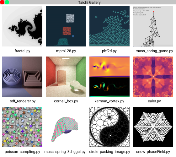
Then click to choose and run the examples.
You can also run the command ti example to view the full list of selected Taichi demos.
Hello, world!
We would like to familiarize you with the Taichi programming language through a basic fractal example, the Julia fractal:
import taichi as ti
import taichi.math as tm

ti.init(arch=ti.gpu)

n = 320
pixels = ti.field(dtype=float, shape=(n * 2, n))

@ti.func
def complex_sqr(z):  # complex square of a 2D vector
    return tm.vec2(z[0] * z[0] - z[1] * z[1], 2 * z[0] * z[1])

@ti.kernel
def paint(t: float):
    for i, j in pixels:  # Parallelized over all pixels
        c = tm.vec2(-0.8, tm.cos(t) * 0.2)
        z = tm.vec2(i / n - 1, j / n - 0.5) * 2
        iterations = 0
        while z.norm() < 20 and iterations < 50:
            z = complex_sqr(z) + c
            iterations += 1
        pixels[i, j] = 1 - iterations * 0.02

gui = ti.GUI("Julia Set", res=(n * 2, n))

for i in range(1000000):
    paint(i * 0.03)
    gui.set_image(pixels)
    gui.show()
To run this program: Save the code above to your disk or execute the command ti example fractal directly in the terminal.
You will see the following animation:
Let's dive into this simple Taichi program.
Import Taichi
import taichi as ti
import taichi.math as tm
The first two lines serve to import Taichi and its math module. The math module contains some frequently used math functions as well as the built-in vectors and matrices of small dimensions, such as vec2 for 2D real vectors and mat3 for 3 x 3 real matrices.
ti.init(arch=ti.gpu)
This line calls the ti.init function to initialize some environment variables. The init function accepts several arguments to allow you to customize your runtime program. For now, we only introduce the most important argument, namely, arch.
The argument arch specifies the backend to execute the compiled code. A backend can be either ti.cpu or ti.gpu. When ti.gpu is designated, Taichi will opt for ti.cuda, ti.vulkan, or ti.opengl/ti.metal in descending order of preference. If no GPU architecture is available, Taichi will fall back to your CPU device.
You can also directly specify the GPU backend by setting, for example, arch=ti.cuda. Taichi will raise an error if the target architecture is unavailable.
Define a field
Let's move on to the next two lines.
n = 320
pixels = ti.field(dtype=float, shape=(n * 2, n))
Here, we define a field whose shape is (640, 320) and whose elements are float-type data. field is the most important and frequently used data structure in Taichi. You can compare it to NumPy's ndarray or PyTorch's tensor. But we need to emphasize that Taichi's field is more powerful and flexible than the two counterparts. For example, a Taichi field can be spatially sparse and can easily switch between different data layouts.
You will come across the advanced features of field in other scenario-based tutorials. For now, it would suffice for you to understand that the field pixels is a dense 2D array.
Kernels and functions
Between Line 9 and Line 22, we define two functions, one decorated with @ti.func and the other with @ti.kernel. They are called the Taichi function and kernel, respectively. Taichi functions and kernels are not executed by Python's interpreter; they are taken over by Taichi's JIT compiler and deployed to your parallel CPU cores or GPU.
The main differences between Taichi functions and kernels:
- Kernels are the entry points where Taichi kicks in and takes over the task. Kernels can be called anywhere, anytime in your program, but Taichi functions can only be called from inside kernels or from inside other Taichi functions. In the example above, the Taichi function
complex_sqris called by the kernelpaint. - A kernel must take type-hinted arguments and return type-hinted results; but Taichi functions do not require type hinting compulsorily. In the example above, the argument
tin the kernelpaintis type hinted, but the argumentzin the Taichi functioncomplex_sqris not. - Taichi supports nested functions but does not support nested kernels. Calling Taichi functions recursively is not supported for now.
tip
For those who come from the world of CUDA, ti.func corresponds to __device__ and ti.kernel corresponds to __global__.
For those who come from the world of OpenGL, ti.func corresponds to the usual function in GLSL and ti.kernel corresponds to a compute shader.
Parallel for loops
The real magic happens at Line 15:
for i, j in pixels:
This is a for loop at the outermost scope in a Taichi kernel and thus is automatically parallelized.
Taichi offers a handy syntax sugar: It parallelizes any for loop at the outermost scope in a kernel. This means that you can parallelize your tasks using just one plain loop, without the need to know what is going on under the hood, be it thread allocation/recycling or memory management.
Note that the field pixels is treated as an iterator. As the indices of the field elements, i and j are integers falling in the ranges [0, 2*n-1] and [0, n-1], respectively. They are arranged in the row-majored order, i.e., (0, 0), (0, 1), ..., (0, n-1), (1, n-1), ..., (2*n-1, n-1).
You should keep it in mind that the for loops not at the outermost scope will not be parallelized; they are handled serially:
@ti.kernel
def fill():
    total = 0
    for i in range(10): # Parallelized
        for j in range(5): # Serialized in each parallel thread
            total += i * j

    if total > 10:
        for k in range(5):  # not parallelized since not at the outermost scope
WARNING
The break statement is not supported in parallelized loops:
@ti.kernel
def foo():
    for i in x:
        ...
        break # Error!

@ti.kernel
def foo():
    for i in x:
        for j in range(10):
            ...
            break # OK!
Display the result
Lines 18-23 render the result on your screen using Taichi's built-in GUI system.
gui = ti.GUI("Julia Set", res=(n * 2, n))

for i in range(1000000):
    paint(i * 0.03)
    gui.set_image(pixels)
    gui.show()
gui = ti.GUI("Julia Set", res=(n * 2, n))
This line sets the window title and the resolution. We plan to iterate over the pixels 1,000,000 times, and the fractal pattern stored in pixels is updated accordingly. Then, we call gui.set_image to set the window and call gui.show() to display the synchronized result on the screen.
Summary
Congratulations! After walking through the above short example, you have learned the most significant features of Taichi:
- Taichi compiles and runs Taichi functions and kernels on the designated backend.
- The
forloop at the outermost scope in a kernel is automatically parallelized. - Taichi provides a powerful and flexible data container
field; you can use indices to loop over afield.
Now, you are well prepared to move on to the more advanced features of Taichi!